최초 NeRF 논문에 대해 코드 리뷰를 해보겠습니다. 논문에서 설명한 내용이 어떻게 구현되어 있는지를 보도록 하겠습니다. 논문에 대한 알고리즘은 [논문 리뷰] NeRF (ECCV2020) : NeRF 최초 논문에 소개되어 있습니다.
NeRF를 구현한 다양한 버전의 오픈소스가 있습니다. pytorch로 구현되어 있는 것 중에서 가장 많은 star를 받은 오픈소스코드를 분석 해보겠습니다.
https://github.com/yenchenlin/nerf-pytorch
GitHub - yenchenlin/nerf-pytorch: A PyTorch implementation of NeRF (Neural Radiance Fields) that reproduces the results.
A PyTorch implementation of NeRF (Neural Radiance Fields) that reproduces the results. - GitHub - yenchenlin/nerf-pytorch: A PyTorch implementation of NeRF (Neural Radiance Fields) that reproduces ...
github.com
NeRF를 개선한 후속 NeRF 논문들에서 부분적으로 해당 코드들을 사용하더군요. 코드를 첨부하다보니 스크롤이 깁니다. 다 읽지 않더라도, 논문을 읽으면서 이해 안되는 부분에 대해서 부분적으로 참고하시면 될 것 같습니다.
아래와 같은 구성으로 소개하겠습니다.
- Data Loading
- Coarse / Fine Sampling
- Rendering
- Loss Function
- MLP
- Positional Encoding
Data Loading
from load_llff import load_llff_data
from load_deepvoxels import load_dv_data
from load_blender import load_blender_data
from load_LINEMOD import load_LINEMOD_data

if args.dataset_type == 'llff':
    images, poses, bds, render_poses, i_test = load_llff_data(args.datadir, args.factor,
                                                              recenter=True, bd_factor=.75,
                                                              spherify=args.spherify)
    hwf, poses = poses[0,:3,-1], poses[:,:3,:4]
    i_val = i_test
    i_train = np.array([i for i in np.arange(int(images.shape[0])) if
                    (i not in i_test and i not in i_val)])
    if args.no_ndc:
        near = np.ndarray.min(bds) * .9
        far = np.ndarray.max(bds) * 1.
    else:
        near = 0.
        far = 1.
elif args.dataset_type == 'blender':
    images, poses, render_poses, hwf, i_split = load_blender_data(args.datadir, args.half_res, args.testskip)
    i_train, i_val, i_test = i_split
    near = 2.
    far = 6.
    if args.white_bkgd:
        images = images[...,:3]*images[...,-1:] + (1.-images[...,-1:])
    else:
        images = images[...,:3]
elif args.dataset_type == 'LINEMOD':
    images, poses, render_poses, hwf, K, i_split, near, far = load_LINEMOD_data(args.datadir, args.half_res, args.testskip)
    i_train, i_val, i_test = i_split
    if args.white_bkgd:
        images = images[...,:3]*images[...,-1:] + (1.-images[...,-1:])
    else:
        images = images[...,:3]
elif args.dataset_type == 'deepvoxels':
    images, poses, render_poses, hwf, i_split = load_dv_data(scene=args.shape,
                                                             basedir=args.datadir,
                                                             testskip=args.testskip)
    i_train, i_val, i_test = i_split
    hemi_R = np.mean(np.linalg.norm(poses[:,:3,-1], axis=-1))
    near = hemi_R-1.
    far = hemi_R+1.
else:
    print('Unknown dataset type', args.dataset_type, 'exiting')
    return
run_nerf.py에서 가장 먼저 데이터를 읽습니다.
dataset type별로 load_xxxx_data.py 파일 입출력 코드가 있습니다. 이를 import합니다.
llff 데이터셋 type은 NeRF 논문에서 "Real Forward-Facing" : fern, trex, orchid, flower, fortress, horns, leaves, room
blender데이터 type은 NeRF논문에서 "Realistic Synthetic 360" : ship, chair, drums, ficus, hotdog, lego, materials, mic
위 파일들에 대해서는 configs폴더에 object별로 config 파일이 작성되어 있습니다.
deepvoxels 데이터 type은 NeRF논문에서 "Diffuse Synthetic 360" 에 해당 하지만 찾지 못했고,
linemode 데이터 type은 논문에서 어떤 것을 의미하는지 모르겠습니다.
images, poses, render_poses, hwf, i_train, i_val, i_test, near, far 이라는 변수를 공통으로 읽어옵니다.
hwf : 이미지의 height, width, focal length를 의미합니다.
poses : 3x4배열 extrinsic matrix로, train시에 rendering할 pose에 해당합니다.
render_poses : 3x5 배열로써 3x4배열까지 extrinsic matrix로 추정되며, inference시에 rendering할 pose에 해당합니다.
near, far : 카메라로부터 Object가 있는 깊이입니다. ray에서 point 샘플링할 최소 최대 깊이를 의미합니다.
i_train, i_val, i_test : train, validation, test에 해당하는 index list입니다.
Coarse Sampling
llff 데이터셋 type의 "fern" scene에 대해 print문을 출력해보았습니다.
K = np.array([
    [focal, 0, 0.5*W],
    [0, focal, 0.5*H],
    [0, 0, 1]
])

def get_rays(H, W, K, c2w): #W는 504, H는 378, c2w는 render_poses
    i, j = torch.meshgrid(torch.linspace(0, W-1, W), torch.linspace(0, H-1, H))
    i = i.t()
    j = j.t() # trans pose
    print(i.shape, j.shape) # torch.Size([378, 504]) torch.Size([378, 504])
    print(i, '\n' , j)
    # tensor([[  0.,   1.,   2.,  ..., 501., 502., 503.],
    #        [  0.,   1.,   2.,  ..., 501., 502., 503.],
    #        [  0.,   1.,   2.,  ..., 501., 502., 503.],
    #        ...,
    #        [  0.,   1.,   2.,  ..., 501., 502., 503.],
    #        [  0.,   1.,   2.,  ..., 501., 502., 503.],
    #        [  0.,   1.,   2.,  ..., 501., 502., 503.]])
    # tensor([[  0.,   0.,   0.,  ...,   0.,   0.,   0.],
    #        [  1.,   1.,   1.,  ...,   1.,   1.,   1.],
    #        [  2.,   2.,   2.,  ...,   2.,   2.,   2.],
    #        ...,
    #        [375., 375., 375.,  ..., 375., 375., 375.],
    #        [376., 376., 376.,  ..., 376., 376., 376.],
    #        [377., 377., 377.,  ..., 377., 377., 377.]])

    dirs = torch.stack([(i-K[0][2])/K[0][0],    #  (i - w/2) / f
    			-(j-K[1][2])/K[1][1],   # -(j - h/2) / f
			-torch.ones_like(i)     # -1
                       ], -1)
    print(dirs.shape) # torch.Size([378, 504, 3])
    print(dirs)
    # tensor([[[-0.6183,  0.4637, -1.0000],
    #     [-0.6159,  0.4637, -1.0000],
    #     [-0.6134,  0.4637, -1.0000],
    #     ...,
    #     [ 0.6109, -0.4613, -1.0000],
    #     [ 0.6134, -0.4613, -1.0000],
    #     [ 0.6159, -0.4613, -1.0000]]])

    rays_d = torch.sum(dirs[..., np.newaxis, :] * c2w[:3,:3], -1)
    rays_o = c2w[:3,-1].expand(rays_d.shape)
    print(rays_d.shape, rays_o.shape) # torch.Size([378, 504, 3]) torch.Size([378, 504, 3])

    return rays_o, rays_d
위의 코드를 통해 pixel 좌표계에 있는 이미지 내 pixel좌표들을 World 좌표계의 voxel좌표로 변환 할 수 있게 합니다.
아래 설명에 대한 용어를 이해하기 위해서 이전 포스트를 읽고 오시길 바랍니다.
[Graphics 기본 개념] - [개념 정리] Camera Intrinsic/Extrinsic Parameters #1
[Graphics 기본 개념] - [개념 정리] Camera Intrinsic/Extrinsic Parameters #2
K배열은 focal length와 principal point의 위치 정보를 갖고 있는 intrinsic matrix입니다.
dirs 배열은 Pixel 좌표계에 있는 pixel들을 camera 좌표계의 normalized plane(카메라 원점으로부터 z거리가 1인)으로 이동한 결과입니다.
c2w배열은 data load시에 읽어온 render_poses에 해당하며, camera 좌표계에 있는 point들을 world 좌표계로 이동시켜주는 camera extrinsic matrix(=world to camera matrix)의 역행렬입니다.
rays_d 배열은 Camera 좌표계의 point들이 world 좌표계로 이동 될 때, 원점을 기준으로 rotation하는 rotation값을 갖고 있는 배열입니다.
rays_o 배열은 Camera 좌표계의 point들이 world 좌표계로 이동 될 때 translation값만 갖고 있는 배열입니다.
rays_d + rays_o를 하면, 카메라를 기준으로한 normalized plane이 world 좌표계 상에서 좌표값을 나타내게 됩니다.
이를 통해, 이미지 plane의 모든 2D좌표들을 Camera Parameter(Intrinsic / Extrinsic) 정보 통해 world 좌표계로 변환시킨 꼴이 됩니다. rays_d와 rays_o를 분리한 이유는 잠시 후에 알 수 있습니다.
    rays_o = torch.reshape(rays_o, [-1,3]).float() # [378,504,3] -> [190512, 3]
    rays_d = torch.reshape(rays_d, [-1,3]).float() # [378,504,3] -> [190512, 3]

    print(near, far) # 0, 1
    near, far = near * torch.ones_like(rays_d[...,:1]), far * torch.ones_like(rays_d[...,:1])

    rays = torch.cat([rays_o, rays_d, near, far], -1)
    print(near.shape, far.shape, rays.shape)
    # [190512, 1] , [190512, 1]) , [190512, 8])
near과 far 각각은 float 1개 값으로 채워진 배열입니다. ones_like는 인자 크기만큼 1로된 배열을 만들어줍니다.
rays에는 World 좌표계 내에서 camera normalized plane의 Voxel 좌표를 표현할 수 있는 rays_d, rays_o 배열과, 최소 깊이값 최대 깊이값을 표현하는 near, far 배열 정보를 저장하고 있게 됩니다.
    N_rays = ray_batch.shape[0]
    rays_o, rays_d = ray_batch[:,0:3], ray_batch[:,3:6] # [N_rays, 3] each
    viewdirs = ray_batch[:,-3:] if ray_batch.shape[-1] > 8 else None
    bounds = torch.reshape(ray_batch[...,6:8], [-1,1,2])
    near, far = bounds[...,0], bounds[...,1] # [-1,1]

    t_vals = torch.linspace(0., 1., steps=N_samples)
    if not lindisp:
        z_vals = near * (1.-t_vals) + far * (t_vals)
    else:
        z_vals = 1./(1./near * (1.-t_vals) + 1./far * (t_vals))

    z_vals = z_vals.expand([N_rays, N_samples])

    if perturb > 0.:
        # get intervals between samples
        mids = .5 * (z_vals[...,1:] + z_vals[...,:-1])
        upper = torch.cat([mids, z_vals[...,-1:]], -1)
        lower = torch.cat([z_vals[...,:1], mids], -1)
        # stratified samples in those intervals
        t_rand = torch.rand(z_vals.shape)

        # Pytest, overwrite u with numpy's fixed random numbers
        if pytest:
            np.random.seed(0)
            t_rand = np.random.rand(*list(z_vals.shape))
            t_rand = torch.Tensor(t_rand)

        z_vals = lower + (upper - lower) * t_rand
ray_batch는 위에서 언급한 rays에 해당합니다. 위에서 서로 다른 값들을 ray 변수를 통해 묶었었는데, 첫 5줄에서는 다시 풀어서 rays_o, rays_d, near, far로 풀어줍니다. (viewdirs설명은 render()쪽에서 설명하겠습니다.)
packing, unpacking이 불필요한 부분이라 생각이 들지만, Batch단위로 연산할 수 있게하고, 코드 가독성을 높여주기 위해 해당 코드가 있는 것이라 생각됩니다.
N_rays는 ray의 갯수를 의미합니다.
N_samples는 1개 ray 위에서 sampling할 point 갯수를 의미합니다.
t_vals는 0~1사이에 N_samples 갯수만큼 사이가 균일하게 나누어진 실수값을 가집니다.
z_vals는 카메라에서 point가 떨어진 깊이를 저장하는 변수입니다. lindisp가 true이면 inverse depth값을 계산하고, False이면 depth값을 계산합니다. lindisp가 False인 경우에 z_vals는 거리가 되며, near부터 far사이의 균일한 값을 저장하게됩니다.
if perturb > 0 : 구간은 논문에서 언급된 stratified sampling에 해당합니다. 균등한 간격의 point를 가진 선위에서, i번째 point위치와 i+1번째 point위치 사이의 랜덤한 위치를 선택하는 sampling 알고리즘입니다.
마지막으로 가장 중요한 코드 부분입니다.
pts = rays_o[...,None,:] + rays_d[...,None,:] * z_vals[...,:,None] # [N_rays, N_samples, 3]rays_o : camera좌표계에서 World좌표계로 이동하는 translation 좌표값
rays_d : Camera좌표계에서 World좌표계로 이동하는 rotation 좌표값
z_vals : Camera좌표계의 원점에서부터 z방향으로 떨어진 거리를 나타내는 깊이 값
으로 위 식을 계산하면,
주어진 Image plane에서 주어진 Camera Pose로 ray를 그렸을 때, World 좌표계에서 Voxel Point 좌표를 알 수 있습니다.
이는 coarse sampling한 point 해당하게 됩니다.
Fine Sampling
    raw = network_query_fn(pts, viewdirs, network_fn)
    rgb_map, disp_map, acc_map, weights, depth_map = raw2outputs(raw, z_vals, rays_d, raw_noise_std, white_bkgd, pytest=pytest)

    if N_importance > 0:
        z_vals_mid = .5 * (z_vals[...,1:] + z_vals[...,:-1])
        z_samples = sample_pdf(z_vals_mid, weights[...,1:-1], N_importance, det=(perturb==0.), pytest=pytest)
        z_samples = z_samples.detach()

        z_vals, _ = torch.sort(torch.cat([z_vals, z_samples], -1), -1)
        pts = rays_o[...,None,:] + rays_d[...,None,:] * z_vals[...,:,None] # [N_rays, N_samples + N_importance, 3]
coarse sampling한 point를 network에 넣고 query한후, weights를 획득합니다. network의 입출력에 대해서 뒤에서 설명하도록하고, 여기서는 fine point sampling을 어떻게 하는지에 대해서 설명하겠습니다.
z_vals_mid는 coarse sampling에서 만든 z_val에서 깊이 중간값을 갖고 옵니다.
N_importance는 1개 ray내 fine sampling할 point갯수 입니다. 128개로 되어있습니다.
sample_pdf함수를 통해 앞선 point좌표에 관한 weight(=volume density)를 사용해서, 확률 밀도 함수에서 point를 샘플링합니다.
Rendering
def render_path(render_poses, hwf, K, chunk, render_kwargs, gt_imgs=None, savedir=None, render_factor=0):
    rgbs, disps = [], []
    for i, c2w in enumerate(tqdm(render_poses)):
        rgb, disp, acc, _ = render(H, W, K, chunk=chunk, c2w=c2w[:3,:4], **render_kwargs)
        rgbs.append(rgb.cpu().numpy())
        disps.append(disp.cpu().numpy())
        if savedir is not None:
            rgb8 = to8b(rgbs[-1])
            filename = os.path.join(savedir, '{:03d}.png'.format(i))
            imageio.imwrite(filename, rgb8)
    rgbs = np.stack(rgbs, 0)
    disps = np.stack(disps, 0)
    return rgbs, disps

rgbs, _ = render_path(render_poses, hwf, K, args.chunk, render_kwargs_test, gt_imgs=images, savedir=testsavedir, render_factor=args.render_factor)
inference에 사용되는 Rendering 코드 부분입니다.
render_path() 함수의 사용되는 핵심 input 인자들은 위에서 준비한 데이터라고 생각하시면 됩니다.
render()함수가 핵심 부분이며, 결과값으로 rgb, disp, acc를 갖습니다.
rgb는 최종 결과 image map를 나타냅니다. png파일로 저장하여 확인 할 수 있습니다.
disp는 disparity map으로써 inverse of depth로 소개되어 있습니다. 코드상 출력해보진 않습니다.
acc는 accumulated opacity(alpha)로 소개되어 있습니다. 또한 코드상 출력해보진 않습니다.
disp와 acc는 실험을 위해 사용되는 parameter로 보입니다.
train에 사용되는 Rendering 코드 부분은, render_path()함수 호출 없이 render() 함수를 batch 단위로 호출합니다.
def render(H, W, K, chunk=1024*32, rays=None, c2w=None, ndc=True,
                  near=0., far=1.,
                  use_viewdirs=False, c2w_staticcam=None,
                  **kwargs):
    ....
    if use_viewdirs:
        viewdirs = rays_d
        viewdirs = viewdirs / torch.norm(viewdirs, dim=-1, keepdim=True)
        viewdirs = torch.reshape(viewdirs, [-1,3]).float()
    ....
    all_ret = batchify_rays(rays, chunk, **kwargs)
....viewdirs는 카메라 pose를 나타냅니다. NeRF논문에서 언급된 MLP의 입력으로 들어가는 view direction값 입니다. 논문과 다른 부분이라면, spherical coordinates를 써서, 2개의 변수(𝜃,𝜙)로 되어있어야 하지만, rays_d의 값을 normalization하여 나누어 3개의 변수로 구성되어 있습니다.
rays는 위에 coarse sampling의 두 번재 코드에서 언급되었습니다. World 좌표계 내에서 camera normalized plane의 Voxel 좌표를 표현할 수 있는 rays_d, rays_o 배열과, 최소 깊이값 최대 깊이값을 표현하는 near, far 배열 정보를 저장하고 있습니다.
all_ret는 rendering결과값을 갖고 있는 변수입니다.
chunk는 한번에 처리할 ray의 갯수입니다. GPU의 Ram크기에 따라 크게 또는 작게 조절 할 수 있습니다.
batchify_rays함수에서 chunk크기로 batch를 만들어 연산합니다.
그 외
use_viewdirs는 view direction을 입력으로 사용할지에 대한 인자입니다.
def batchify_rays(rays_flat, chunk=1024*32, **kwargs):
    all_ret = {}
    for i in range(0, rays_flat.shape[0], chunk):
        ret = render_rays(rays_flat[i:i+chunk], **kwargs)
        for k in ret:
            if k not in all_ret:
                all_ret[k] = []
            all_ret[k].append(ret[k])

    all_ret = {k : torch.cat(all_ret[k], 0) for k in all_ret}
return all_retrays_flat은 위에 코드에서 언급한 rays에 해당합니다.
render_rays는 ray_flat을 입력으로, ray위에 있는 voxel들의 color와 volume density를 출력으로 갖는 함수 입니다.
chuck 크기 만큼 batch로 구성하여, render_rays 함수를 수행한 후에, 결과값을 all_ret이라는 자료구조로 저장하는 코드입니다.
def render_rays(ray_batch,
                network_fn,
                network_query_fn,
                N_samples,
                retraw=False,
                lindisp=False,
                perturb=0.,
                N_importance=0,
                network_fine=None,
                white_bkgd=False,
                raw_noise_std=0.,
                verbose=False,
                pytest=False):

    ........
    pts = rays_o[...,None,:] + rays_d[...,None,:] * z_vals[...,:,None] # [N_rays, N_samples, 3]
    raw = network_query_fn(pts, viewdirs, network_fn)
    rgb_map, disp_map, acc_map, weights, depth_map = raw2outputs(raw, z_vals, rays_d, raw_noise_std, white_bkgd, pytest=pytest)

    if N_importance > 0:
        ........
        z_samples = sample_pdf(z_vals_mid, weights[...,1:-1], N_importance, det=(perturb==0.), pytest=pytest)
        z_vals, _ = torch.sort(torch.cat([z_vals, z_samples], -1), -1)
        pts = rays_o[...,None,:] + rays_d[...,None,:] * z_vals[...,:,None] # [N_rays, N_samples + N_importance, 3]

        run_fn = network_fn if network_fine is None else network_fine
        raw = network_query_fn(pts, viewdirs, run_fn)

        rgb_map, disp_map, acc_map, weights, depth_map = raw2outputs(raw, z_vals, rays_d, raw_noise_std, white_bkgd, pytest=pytest)

    ......
    ret = {'rgb_map' : rgb_map, 'disp_map' : disp_map, 'acc_map' : acc_map}
    return ret
첫번째 pts는 coarse sampling의 point값 입니다. 그리고 두번째 연급된 pts는 fine sampling의 point 값입니다.
network_query_fn()함수는 pts와 view direction값을 입력으로 하여, raw라는 출력값을 갖는 MLP 함수입니다. Network의 결과값을 post process없이 그대로 출력한다는 의미로 raw라는 변수명을 붙인 것 같습니다.
raw2outputs()함수는 raw를 입력으로 하여, rgb_map, disp_map, acc_map, weights, depth_map형태로 변환하는 후처리 함수입니다. NeRF논문에서 volume rendering 수식이 들어가는 부분입니다.
N_importance는 fine sampling할 point 갯수입니다.
첫번째 network_query_fn()함수는 논문에서 coarse network에 해당하고, 두번째 network_query_fn()함수는 논문에서 fine entwork에 해당합니다.
여기 코드에서 주요하게 볼 부분은
- coarse network의 결과 값인 weight로 fine network의 입력값을 계산한다는 점
- fine network의 결과 값이 coarse network의 결과값을 덮어버린다는 점
입니다. 논문에서 final rendering color는 fine network의 결과로 사용한다고 되어 있고 이 부분이 코드에 반영되어 있는 것을 확인해 볼 수 있습니다.
def batchify(fn, chunk):
    def ret(inputs):
        return torch.cat([fn(inputs[i:i+chunk]) for i in range(0, inputs.shape[0], chunk)], 0)
    return ret

def run_network(inputs, viewdirs, fn, embed_fn, embeddirs_fn, netchunk=1024*64):
    """Prepares inputs and applies network 'fn'.
    """
    inputs_flat = torch.reshape(inputs, [-1, inputs.shape[-1]])
    embedded = embed_fn(inputs_flat)

    if viewdirs is not None:
        input_dirs = viewdirs[:,None].expand(inputs.shape)
        input_dirs_flat = torch.reshape(input_dirs, [-1, input_dirs.shape[-1]])
        embedded_dirs = embeddirs_fn(input_dirs_flat)
        embedded = torch.cat([embedded, embedded_dirs], -1)

    outputs_flat = batchify(fn, netchunk)(embedded)
    outputs = torch.reshape(outputs_flat, list(inputs.shape[:-1]) + [outputs_flat.shape[-1]])
return outputsembeddirs_fn()함수는 positional encoding부분이며, 아래에서 설명하겠습니다.
batchify()함수는 단순한 반복수행 명령문에 해당하고, 인자인 fn이 network의 forward함수에 해당합니다. 아래 MLP 부분에서 설명하겠습니다.
run_network()함수를 통해 network의 결과값을 post process없이 return합니다.
def raw2outputs(raw, z_vals, rays_d, raw_noise_std=0, white_bkgd=False, pytest=False):
    raw2alpha = lambda raw, dists, act_fn=F.relu: 1.-torch.exp(-act_fn(raw)*dists)

    dists = z_vals[...,1:] - z_vals[...,:-1]
    dists = torch.cat([dists, torch.Tensor([1e10]).expand(dists[...,:1].shape)], -1)  # [N_rays, N_samples]

    dists = dists * torch.norm(rays_d[...,None,:], dim=-1)

    rgb = torch.sigmoid(raw[...,:3])  # [N_rays, N_samples, 3]
    noise = 0.
    if raw_noise_std > 0.:
        noise = torch.randn(raw[...,3].shape) * raw_noise_std
        # Overwrite randomly sampled data if pytest
        if pytest:
            np.random.seed(0)
            noise = np.random.rand(*list(raw[...,3].shape)) * raw_noise_std
            noise = torch.Tensor(noise)

    alpha = raw2alpha(raw[...,3] + noise, dists)  # [N_rays, N_samples]
    # weights = alpha * tf.math.cumprod(1.-alpha + 1e-10, -1, exclusive=True)
    weights = alpha * torch.cumprod(torch.cat([torch.ones((alpha.shape[0], 1)), 1.-alpha + 1e-10], -1), -1)[:, :-1]
    rgb_map = torch.sum(weights[...,None] * rgb, -2)  # [N_rays, 3]

    depth_map = torch.sum(weights * z_vals, -1)
    disp_map = 1./torch.max(1e-10 * torch.ones_like(depth_map), depth_map / torch.sum(weights, -1))
    acc_map = torch.sum(weights, -1)

    if white_bkgd:
        rgb_map = rgb_map + (1.-acc_map[...,None])

return rgb_map, disp_map, acc_map, weights, depth_mapdists는 ray위에서 있는 point간의 거리를 나타냅니다. rays_d를 사용하여 rotation을 시켜, 카메라 좌표계에 있는 Point들을 World 좌표계로 이동 시켜줍니다.
rgb는 MLP의 출력인 raw에서 앞쪽 3개에 해당하는 값 입니다.
noise는 Gaussian Noise로 생성되어집니다. 눈문 Appendix A. Training Details에 가우시안 노이즈를 적용해서 약간의 퀄리티 향상을 할 수 있었다고 합니다. torch.randn는 평균이 0이고 표준편차가 1인 가우시안 분포 즉 Standard Normal Distribution을 만드는 함수입니다. raw_noise_std는 가우시안 분포의 표준 편차(standard deviataion)에 해당합니다.
alpha는 아래 (1-exp(-𝜎𝑖δi))에 해당하는 값이므로, MLP출력값인 raw의 volume density값과 dists값의 곱으로 계산되며 Target Point의 불투명도를 나타냅니다. exp(-𝜎𝑖δi) 는 투명도를 나타내고, 1-exp(-𝜎𝑖δi) 는 불투명도(알파값)를 나타냅니다. 0이면 투명하고 1이면 불투명한 값을 나타냅니다.

weights는 Ti*(1-exp(-𝜎𝑖δi))에 해당하는 값이며, 카메라에서 Target Point i 까지의 영역에 대한 투명도를 나타내는 Ti값과 Target Point i에서의 불투명도를 나타내는 alpha값이 곱해집니다. crumprod는 누적곱을 의미하며, j는 1부터 i-1까지의 투명도를 누적곱하게 됩니다. 의미는 카메라로 i번째 Point를 바라봤을 때, i번째 Point의 영향도(=가중치)를 나타냅니다.
rgb_map은 C(r)에 해당하는 값입니다. ray위의 N개의 모든 점에 대해 summation하여 계산합니다. sum( weights * rgb ) 으로 표현되어 있습니다.
depth_map은 weights와 z_vals(Camera좌표계의 원점에서부터 z방향으로 떨어진 거리를 나타내는 깊이 값)를 곱하고 전체를 summation함으로써, Volume Density 값으로 Depth Map을 형성합니다. 위의 C(r)식에서 ci 대신에 z_vals가 들어갔다고 보시면 됩니다. 카메라로부터 멀수록 값이 커지고, weight인 Ti*(1-exp(-𝜎𝑖δi)) 가 클수록 값이 커집니다.
disp_map은 disparity map이며, 제가 알고 있는 disparity map은 Stereo 이미지에서 객체의 위치 상의 다른 차이를 나타낸 map인데, 여기에서는 depth map을 inverse한 map으로 표현되어 있습니다. depth가 너무 작을 경우(=물체가 카메라에 너무 가까이 있을 경우) disparity는 exp(10) = 22026.465 의 값인 아주 큰 값을 갖게 되고, 그 외의 경우에는
disp_map는 torch.sum(weights, -1) / depth_map 의 값을 가지게 됩니다.
depth_map은 torch.sum(weights * z_vals, -1) 이었기 때문에,
disp_map은 torch.sum(weights, -1) / torch.sum(weights * z_vals, -1) 이므로, 아래 수식으로 표현 할 수 있습니다.

z_vals는 Camera좌표계의 원점에서부터 z방향으로 떨어진 거리를 나타내는 깊이 값을 나타냈었습니다.
acc_map은 accumulated map으로써, weights들을 summation하여 나타냅니다. fine network의 입력값들을 Sampling할 때 사용됩니다.
Loss Function
    img2mse = lambda x, y : torch.mean((x - y) ** 2)
    mse2psnr = lambda x : -10. * torch.log(x) / torch.log(torch.Tensor([10.]))

    ......
    start = start + 1
    for i in trange(start, N_iters):
        ......
        rgb, disp, acc, extras = render(H, W, K, chunk=args.chunk, rays=batch_rays,
                                                verbose=i < 10, retraw=True,
                                                **render_kwargs_train)
        optimizer.zero_grad()
        img_loss = img2mse(rgb, target_s)
        trans = extras['raw'][...,-1]
        loss = img_loss
        psnr = mse2psnr(img_loss)

        if 'rgb0' in extras:
            img_loss0 = img2mse(extras['rgb0'], target_s)
            loss = loss + img_loss0
            psnr0 = mse2psnr(img_loss0)

        loss.backward()
        optimizer.step()
loss는 predicted rgb결과값과 ground truth 이미지(=targets) 대한 mean square error를 계산합니다.
rgb는 fine network로 rendering한 이미지를 나타냅니다.
extras['rgb0']는 coarse network로 rendering한 이미지를 나타냅니다.
coarse network, fine network 각각에 대해 loss를 구하고 더한 후에, back propagation 하는 것을 볼 수 있습니다.
MLP
def create_nerf(args):

    model = NeRF(D=args.netdepth, W=args.netwidth,
                 input_ch=input_ch, output_ch=output_ch, skips=skips,
                 input_ch_views=input_ch_views, use_viewdirs=args.use_viewdirs).to(device)
    grad_vars = list(model.parameters())

    model_fine = None
    if args.N_importance > 0:
        model_fine = NeRF(D=args.netdepth_fine, W=args.netwidth_fine,
                          input_ch=input_ch, output_ch=output_ch, skips=skips,
                          input_ch_views=input_ch_views, use_viewdirs=args.use_viewdirs).to(device)
grad_vars += list(model_fine.parameters())model은 coarse network를 의미하고
model_fine은 fine network를 의미합니다.
class NeRF(nn.Module):
def __init__(self, D=8, W=256, input_ch=3, input_ch_views=3, output_ch=4, skips=[4], use_viewdirs=False):
super(NeRF, self).__init__()
self.D = D
self.W = W
self.input_ch = input_ch
self.input_ch_views = input_ch_views
self.skips = skips
self.use_viewdirs = use_viewdirs
self.pts_linears = nn.ModuleList(
[nn.Linear(input_ch, W)] + [nn.Linear(W, W) if i not in self.skips else nn.Linear(W + input_ch, W) for i in range(D-1)])
self.views_linears = nn.ModuleList([nn.Linear(input_ch_views + W, W//2)])
if use_viewdirs:
self.feature_linear = nn.Linear(W, W)
self.alpha_linear = nn.Linear(W, 1)
self.rgb_linear = nn.Linear(W//2, 3)
else:
self.output_linear = nn.Linear(W, output_ch)
def forward(self, x):
input_pts, input_views = torch.split(x, [self.input_ch, self.input_ch_views], dim=-1)
h = input_pts
for i, l in enumerate(self.pts_linears):
h = self.pts_linears[i](h)
h = F.relu(h)
if i in self.skips:
h = torch.cat([input_pts, h], -1)
if self.use_viewdirs:
alpha = self.alpha_linear(h)
feature = self.feature_linear(h)
h = torch.cat([feature, input_views], -1)
for i, l in enumerate(self.views_linears):
h = self.views_linears[i](h)
h = F.relu(h)
rgb = self.rgb_linear(h)
outputs = torch.cat([rgb, alpha], -1)
else:
outputs = self.output_linear(h)
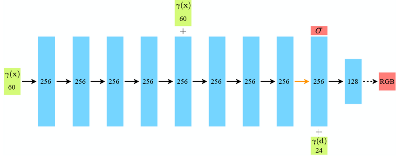
return outputs논문에 언급된 아래 네트워크를 구현한 코드입니다.
use_viewdirs는 모두 true로 되어 있습니다. skip connection, relu가 쓰이는 것을 볼 수 있습니다.
Positional Encoding
# Positional encoding (section 5.1)
class Embedder:
    def __init__(self, **kwargs):
        self.kwargs = kwargs
        self.create_embedding_fn()

    def create_embedding_fn(self):
        embed_fns = []
        d = self.kwargs['input_dims']
        out_dim = 0
        if self.kwargs['include_input']:
            embed_fns.append(lambda x : x)
            out_dim += d

        max_freq = self.kwargs['max_freq_log2']
        N_freqs = self.kwargs['num_freqs']

        if self.kwargs['log_sampling']:
            freq_bands = 2.**torch.linspace(0., max_freq, steps=N_freqs)
        else:
            freq_bands = torch.linspace(2.**0., 2.**max_freq, steps=N_freqs)

        for freq in freq_bands:
            for p_fn in self.kwargs['periodic_fns']:
                embed_fns.append(lambda x, p_fn=p_fn, freq=freq : p_fn(x * freq))
                out_dim += d

        self.embed_fns = embed_fns
        self.out_dim = out_dim

    def embed(self, inputs):
        return torch.cat([fn(inputs) for fn in self.embed_fns], -1)
def get_embedder(multires, i=0):
if i == -1:
return nn.Identity(), 3
embed_kwargs = {
'include_input' : True,
'input_dims' : 3,
'max_freq_log2' : multires-1,
'num_freqs' : multires,
'log_sampling' : True,
'periodic_fns' : [torch.sin, torch.cos],
}
embedder_obj = Embedder(**embed_kwargs)
embed = lambda x, eo=embedder_obj : eo.embed(x)
return embed, embedder_obj.out_dimEmbedder라는 class를 생성할 때, periodic_fns에서 sin, cos 함수가 들어갑니다.
이 값은 create_embedding_fn 함수내 2중 for문이 하나 있는데, 여기서 아래 수식을 만듧니다.

Closing...
NeRF의 Original 논문에 대해 코드 분석을 해봤습니다. 위에 코드들은 실제로 2개의 python 파일로 되어 있습니다. 다 합쳐도 1000줄이 되지 않습니다. 비교적 짧은? 코드로 깔끔하게 구현 되어 있습니다. 논문에 언급 안된 실험적인 코드 들이 분기문으로 되어 있었으나 설명을 생략하고 지나갔습니다. 역시 논문에서 언급한대로 시간이 오래걸리네요. GPU없이 i7 8세대 CPU로 이미지 378x504해상도 1장 inference에 9분 45초 소요되었습니다...후속 NeRF논문들에서 해당 코드를 참조하는 형태로 쓰고 있어서, 다른 코드 분석시에는 다른 점만 언급하면 될 것 같네요.
'NeRF' 카테고리의 다른 글
| [논문 리뷰] NeRF-W (CVPR 2021) : Uncertainty 접목 연구 (0) | 2022.12.13 |
|---|---|
| [논문 리뷰] Mip-NeRF (CVPR 2021) : Anti-Aliasing 연구 (2) | 2022.12.04 |
| [논문 리뷰] BARF (ICCV 2021) : Unknown 카메라 pose에서 NeRF (1) | 2022.11.24 |
| [논문 리뷰] Instant NGP(SIGGRAPH 2022) : 인코딩 방법 개선으로 속도 향상 (2) | 2022.11.10 |
| [논문 리뷰] MVSNeRF (ICCV2021) : 적은 입력 + 학습 속도 개선 논문 (0) | 2022.10.27 |


댓글